Custom Soil Emission Factors

Creating custom emission factors to assess soil carbon stock using multiple management practices. These custom emission factors were ran using linear mixed effect modeling practices shown in the R Script below.

#Estimating Emission Factors using a linear mixed effect model (LME)

  #LME model using backwards stepwise method

  #Using mixed effect model because we have fixed and random variables

#----load nlme package (linear and non linear mixed effects model)-----

library(nlme)

#----Read in EF input file----

LU.data<-read.csv("data/SoilCCult.csv", header=TRUE)

management.data<-read.csv("data/SoilCManagement.csv", header=TRUE)

Cinput.data<-read.csv("data/SoilCInput.csv", header=TRUE)

#-----Test for correlation in predictor variables-------

cor(LU.data[,c("years", "years2", "dep1", "dep2")])

             years      years2       dep1         dep2
years  1.000000000  0.94730657 0.02220118  0.001486767
years2 0.947306573  1.00000000 0.01113563 -0.013561348
dep1   0.022201178  0.01113563 1.00000000  0.928455277
dep2   0.001486767 -0.01356135 0.92845528  1.000000000

cor(management.data[,c("years", "years2", "dep1", "dep2")])

           years    years2      dep1      dep2
years  1.0000000 0.9641991 0.2098040 0.2105650
years2 0.9641991 1.0000000 0.2086141 0.2123727
dep1   0.2098040 0.2086141 1.0000000 0.9513001
dep2   0.2105650 0.2123727 0.9513001 1.0000000

cor(Cinput.data[,c("years", "years2", "dep1", "dep2")])

           years    years2      dep1      dep2
years  1.0000000 0.9778155 0.1705907 0.1374545
years2 0.9778155 1.0000000 0.1705167 0.1358530
dep1   0.1705907 0.1705167 1.0000000 0.9557745
dep2   0.1374545 0.1358530 0.9557745 1.0000000

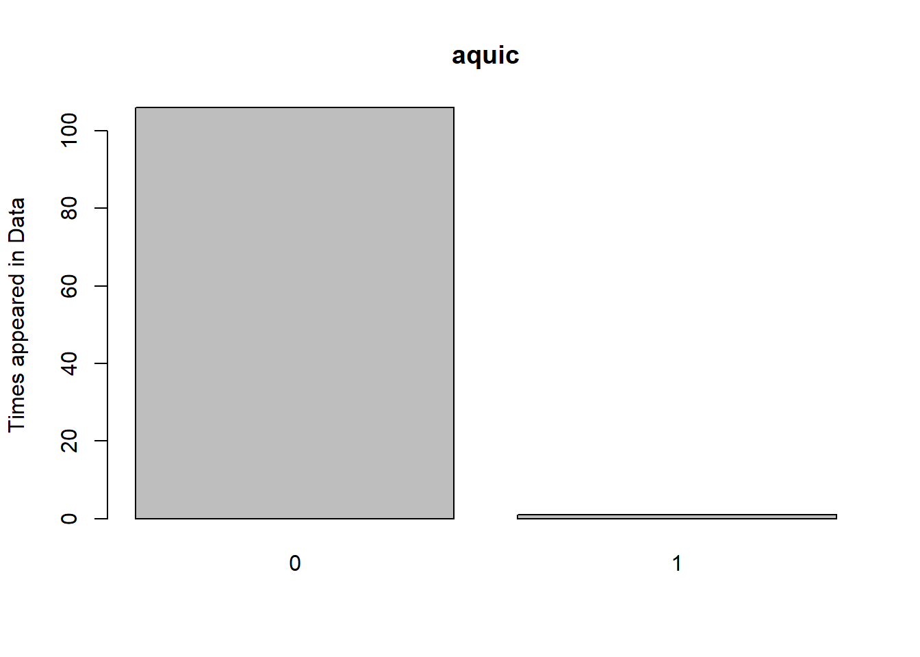
#----Data check via Visualization----

###Aquic

barplot(table(Cinput.data$aquic),ylab = "Times appeared in Data", main= "aquic")

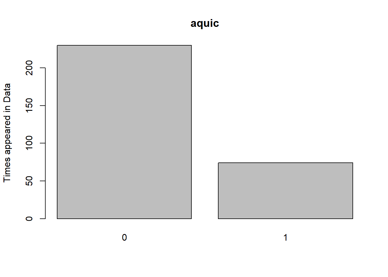
barplot(table(management.data$aquic),ylab = "Times appeared in Data", main= "aquic")

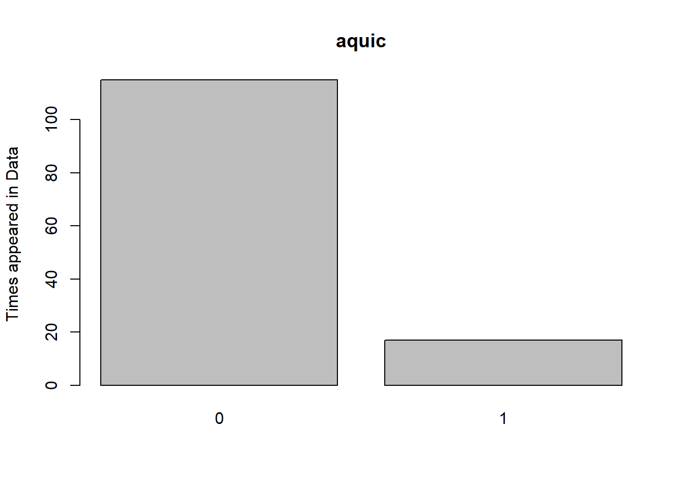
barplot(table(LU.data$aquic),ylab = "Times appeared in Data", main= "aquic")

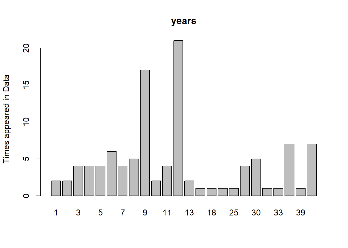
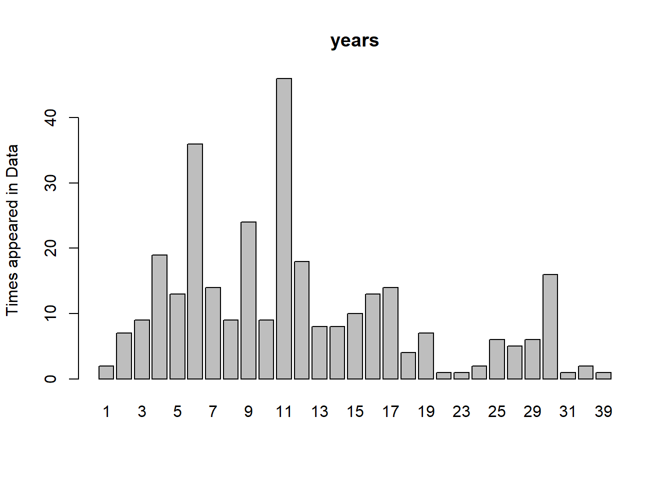
###Years and Years2 (years squared)

barplot(table(Cinput.data$years),ylab = "Times appeared in Data", main= "years")

barplot(table(management.data$years),ylab = "Times appeared in Data", main= "years")

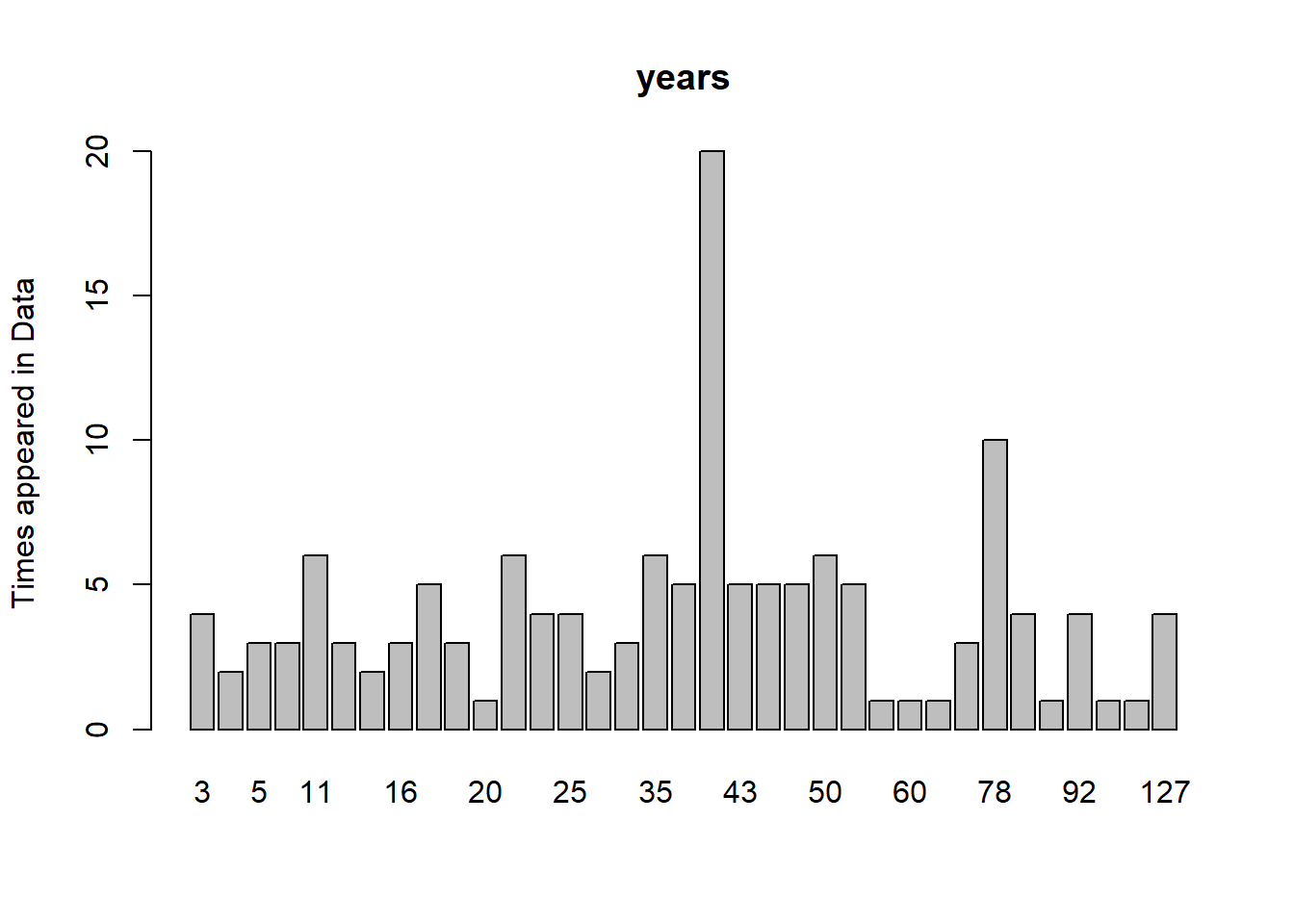
barplot(table(LU.data$years),ylab = "Times appeared in Data", main= "years")

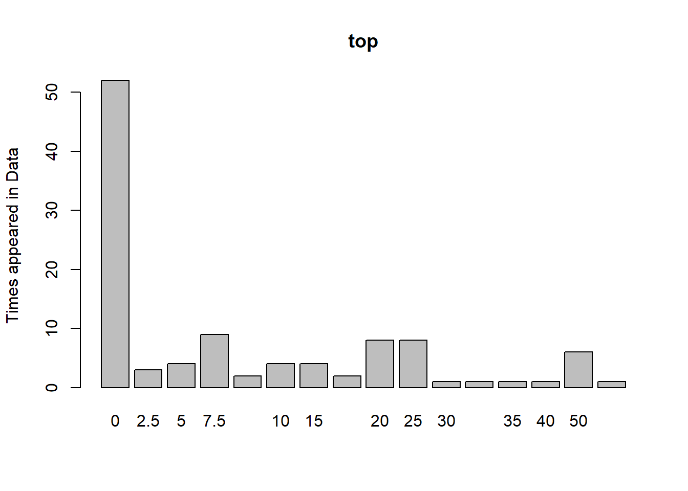
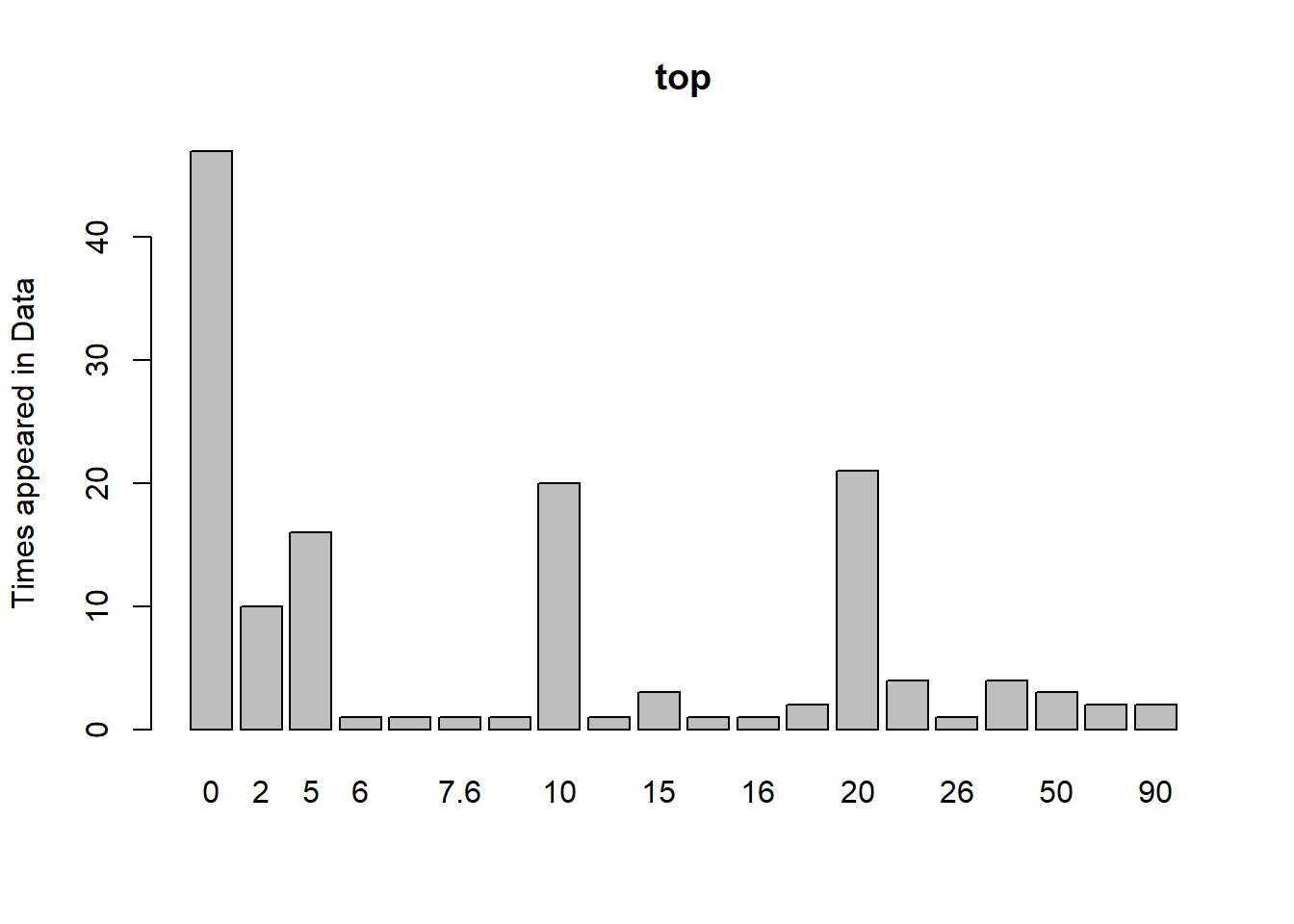
###Top and bottom

barplot(table(Cinput.data$top),ylab = "Times appeared in Data", main= "top")

barplot(table(management.data$top),ylab = "Times appeared in Data", main= "top")

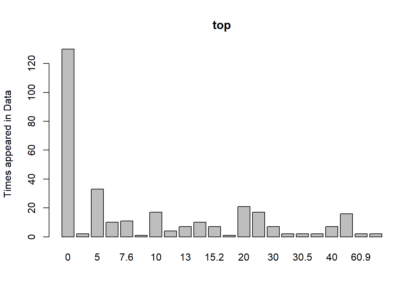
barplot(table(LU.data$top),ylab = "Times appeared in Data", main= "top")

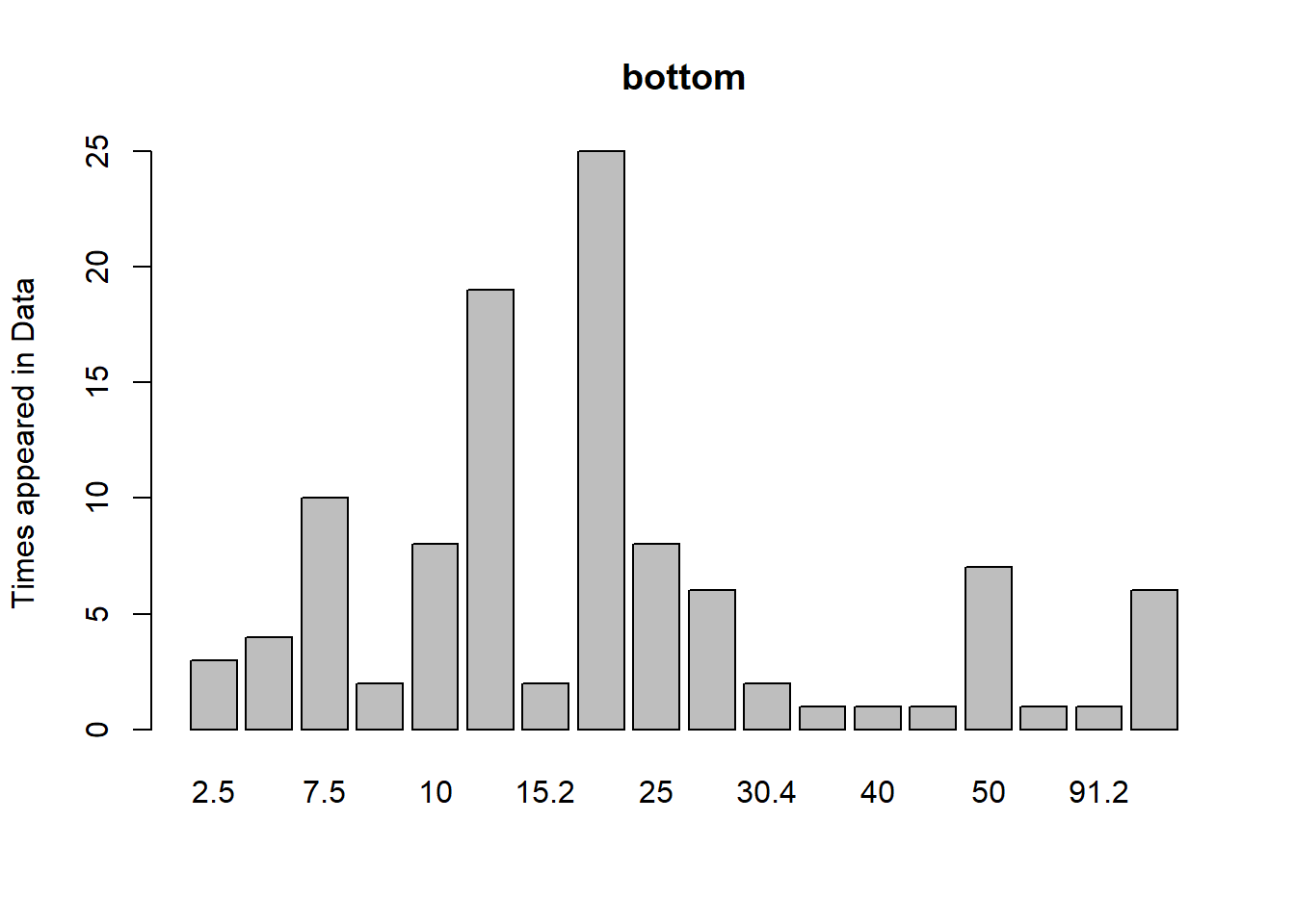
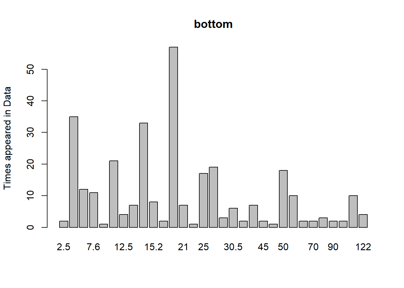
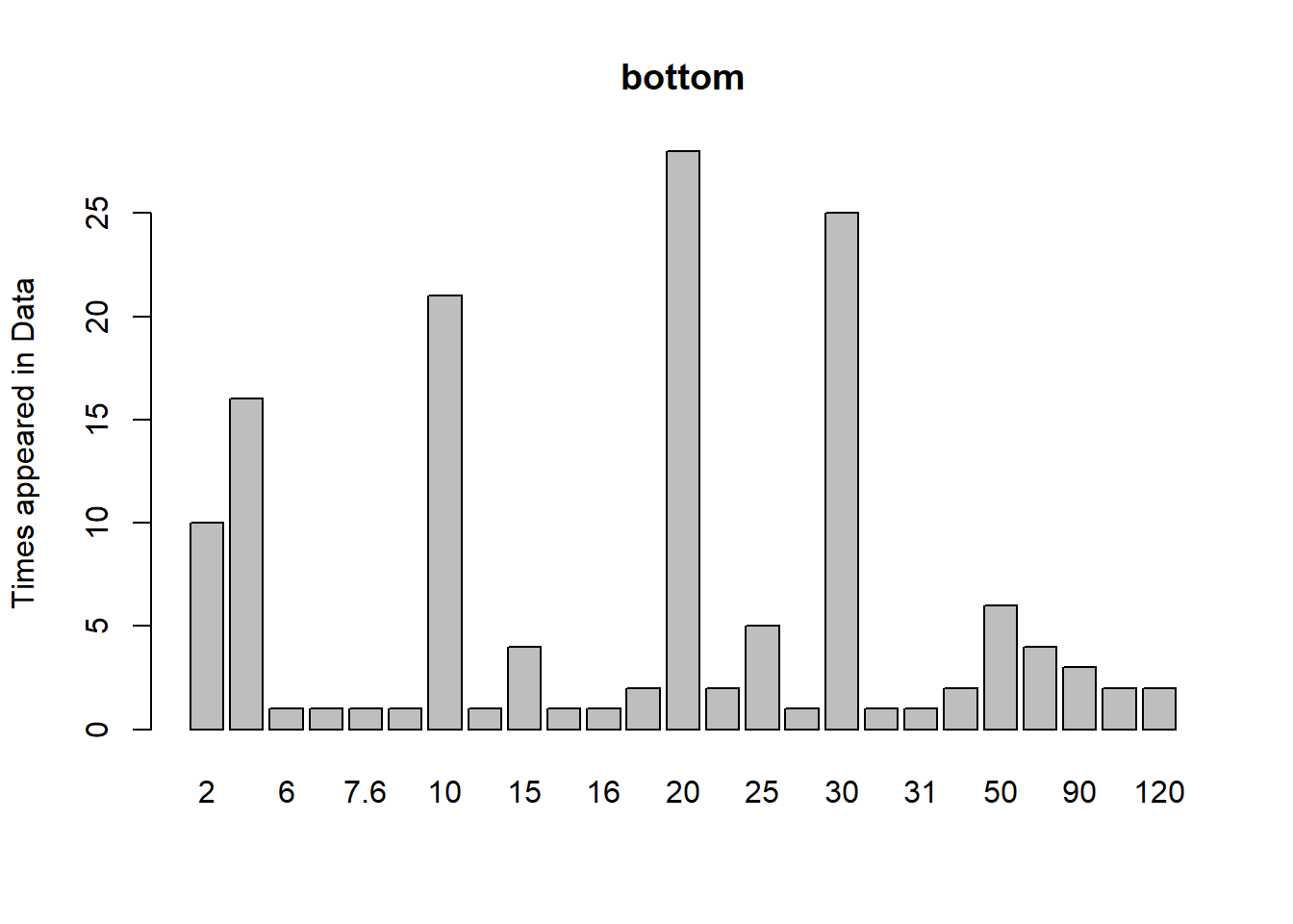
barplot(table(Cinput.data$bottom),ylab = "Times appeared in Data", main= "bottom")

barplot(table(management.data$bottom),ylab = "Times appeared in Data", main= "bottom")

barplot(table(LU.data$bottom),ylab = "Times appeared in Data", main= "bottom")

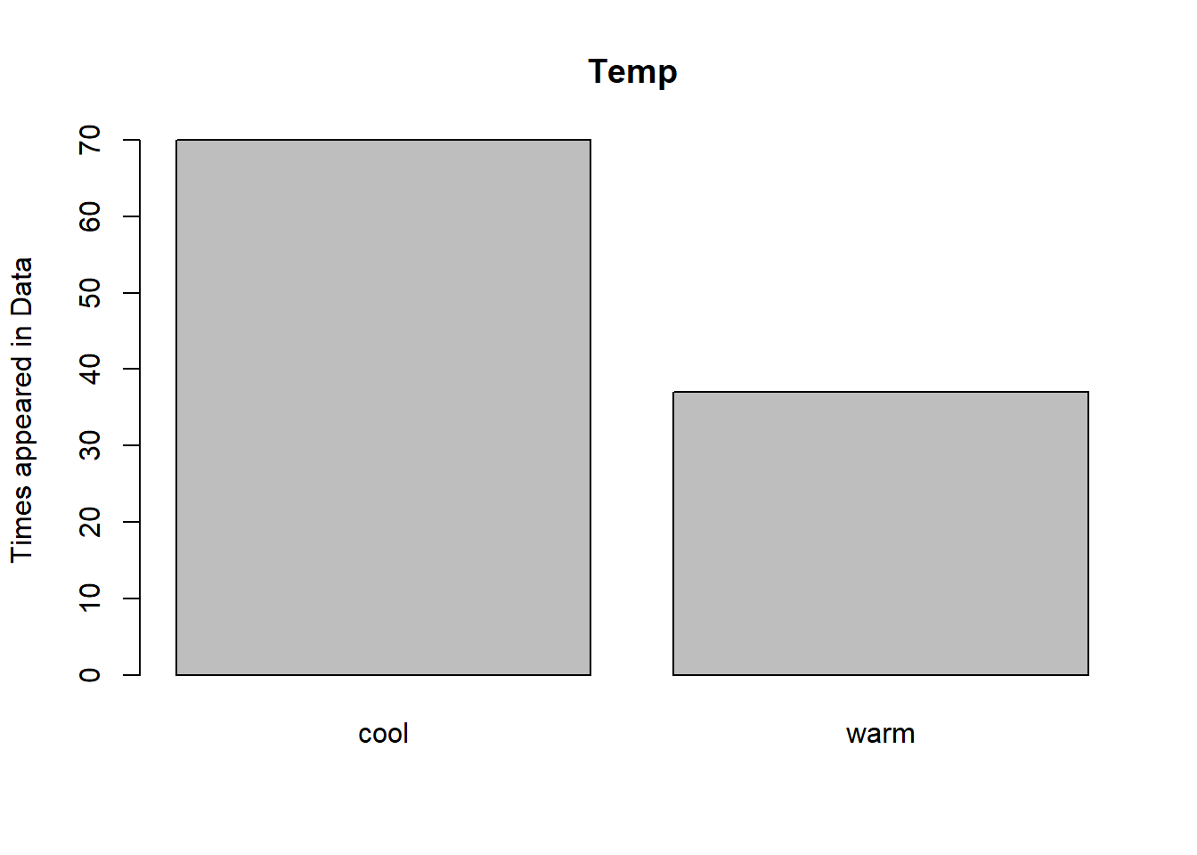
###Temp

barplot(table(Cinput.data$ipcc.temp),ylab = "Times appeared in Data", main= "Temp")

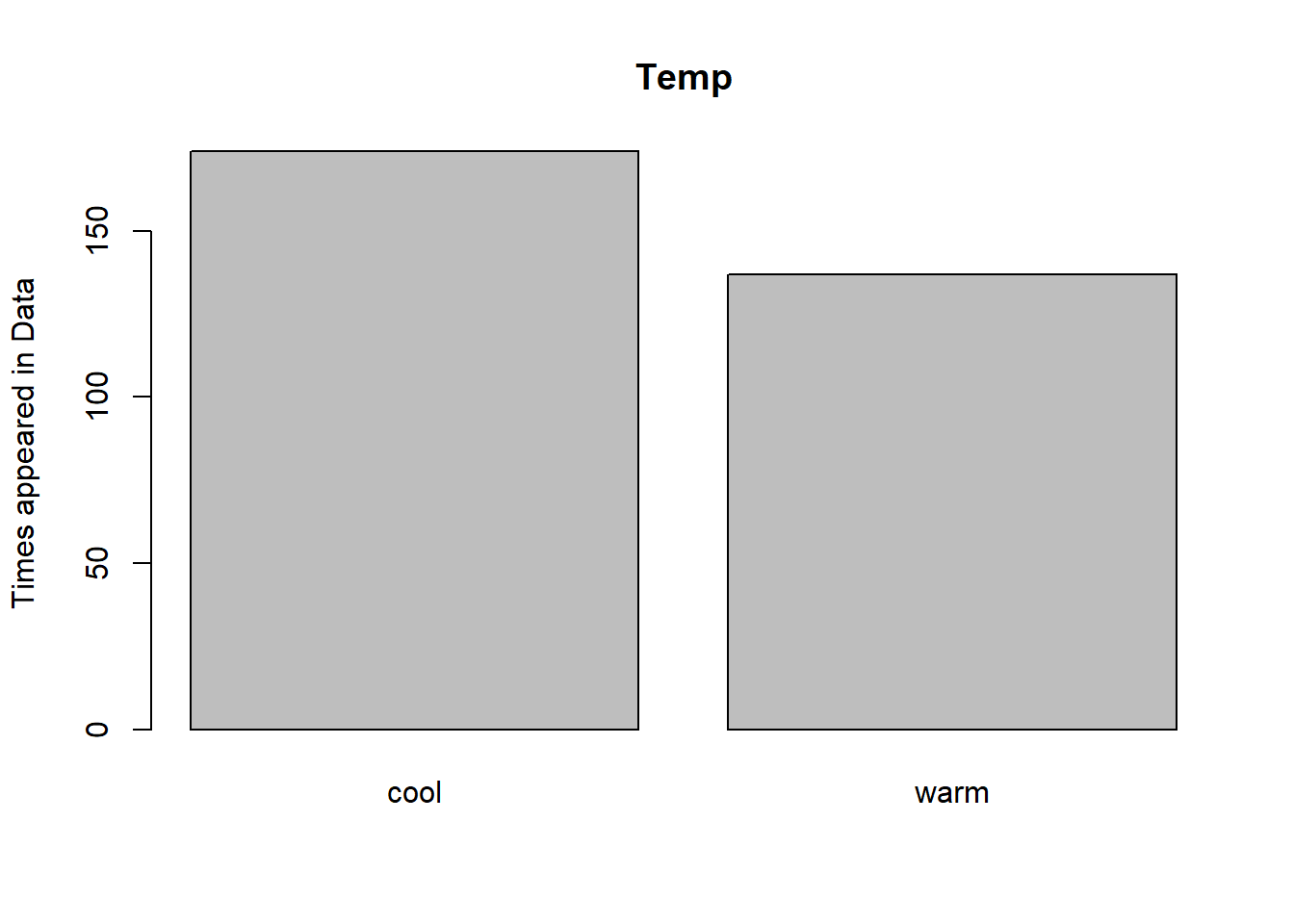
barplot(table(management.data$ipcc.temp),ylab = "Times appeared in Data", main= "Temp")

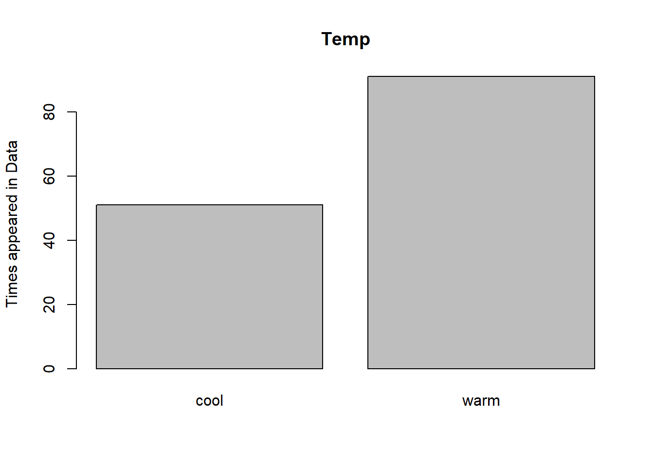
barplot(table(LU.data$ipcc.temp),ylab = "Times appeared in Data", main= "Temp")

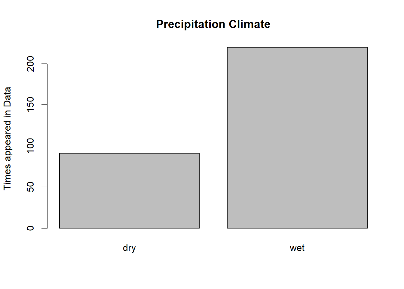
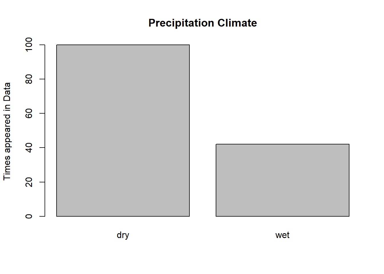
###Precipitation

barplot(table(Cinput.data$ipcc.pre),ylab = "Times appeared in Data", main= "Precipitation Climate")

barplot(table(management.data$ipcc.pre),ylab = "Times appeared in Data", main= "Precipitation Climate")

barplot(table(LU.data$ipcc.pre),ylab = "Times appeared in Data", main= "Precipitation Climate")

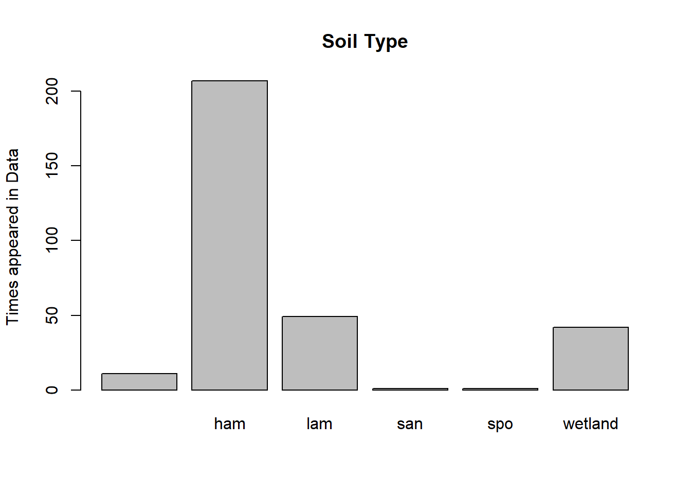
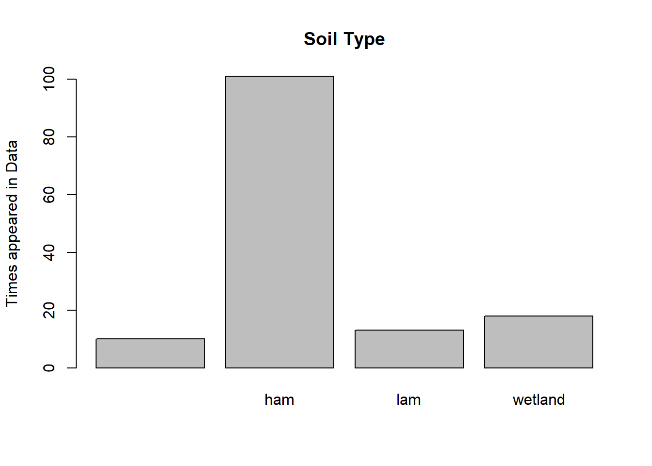
###Soil type

barplot(table(Cinput.data$ipcc.soil),ylab = "Times appeared in Data", main= "Soil Type")

barplot(table(management.data$ipcc.soil),ylab = "Times appeared in Data", main= "Soil Type")

barplot(table(LU.data$ipcc.soil),ylab = "Times appeared in Data", main= "Soil Type")

#_____________________________________________________________________________________________________

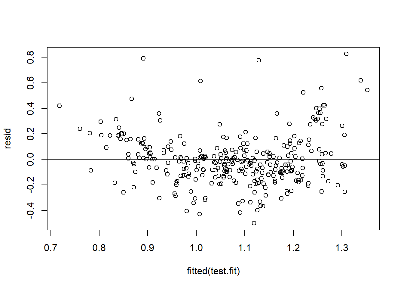
  #MANAGEMENT MODEL DEVELOPMENT

#-------Test full model with all variables as main effects-------

test.fit<-lme(ch.cstock~ch.till+years+years2+dep1+dep2+aquic+ipcc.soil+ipcc.pre+ipcc.temp,

              random = ~1|ran.exp/ran.yrexp, data = management.data, method = "ML", na.action = na.omit)

summary(test.fit)

Linear mixed-effects model fit by maximum likelihood
  Data: management.data 
        AIC       BIC   logLik
  -74.82665 -11.80577 54.41332

Random effects:
 Formula: ~1 | ran.exp
         (Intercept)
StdDev: 2.888098e-05

 Formula: ~1 | ran.yrexp %in% ran.exp
        (Intercept)  Residual
StdDev: 2.98371e-05 0.2019543

Fixed effects:  ch.cstock ~ ch.till + years + years2 + dep1 + dep2 + aquic +      ipcc.soil + ipcc.pre + ipcc.temp 
                      Value  Std.Error  DF   t-value p-value
(Intercept)       1.2052050 0.12792012 197  9.421544  0.0000
ch.tillrt        -0.0424258 0.02644707 197 -1.604176  0.1103
years             0.0034526 0.00673113  30  0.512933  0.6118
years2           -0.0000308 0.00018991  30 -0.162072  0.8723
dep1             -0.0214199 0.00223077 197 -9.602025  0.0000
dep2              0.0002240 0.00002812 197  7.966228  0.0000
aquic            -0.0038566 0.04172614  60 -0.092427  0.9267
ipcc.soilham      0.0294098 0.10978879  60  0.267876  0.7897
ipcc.soillam     -0.0166472 0.11363556  60 -0.146497  0.8840
ipcc.soilsan     -0.0365804 0.23503276  60 -0.155639  0.8768
ipcc.soilspo     -0.0318737 0.23362227  60 -0.136433  0.8919
ipcc.soilwetland  0.0219131 0.11953004  60  0.183327  0.8552
ipcc.prewet       0.0890616 0.03076183  60  2.895199  0.0053
ipcc.tempwarm     0.0017827 0.03373953  60  0.052837  0.9580
 Correlation: 
                 (Intr) ch.tll years  years2 dep1   dep2   aquic  ipcc.slh
ch.tillrt         0.043                                                   
years            -0.387 -0.006                                            
years2            0.356 -0.019 -0.965                                     
dep1             -0.185 -0.099 -0.020  0.032                              
dep2              0.140  0.085  0.039 -0.063 -0.952                       
aquic             0.087 -0.053 -0.114  0.145  0.043 -0.071                
ipcc.soilham     -0.910 -0.104  0.077 -0.073  0.048 -0.021 -0.078         
ipcc.soillam     -0.877 -0.058  0.251 -0.217  0.099 -0.051 -0.052  0.900  
ipcc.soilsan     -0.440 -0.012  0.111 -0.096 -0.018  0.022 -0.004  0.455  
ipcc.soilspo     -0.413 -0.011  0.034 -0.025 -0.017  0.021  0.004  0.452  
ipcc.soilwetland -0.831 -0.071  0.163 -0.171  0.022  0.008 -0.369  0.895  
ipcc.prewet      -0.242  0.043 -0.022  0.001 -0.208  0.191 -0.265  0.162  
ipcc.tempwarm    -0.144 -0.048 -0.362  0.317  0.082 -0.102  0.067  0.191  
                 ipcc.sll ipcc.slsn ipcc.slsp ipcc.slw ipcc.p
ch.tillrt                                                    
years                                                        
years2                                                       
dep1                                                         
dep2                                                         
aquic                                                        
ipcc.soilham                                                 
ipcc.soillam                                                 
ipcc.soilsan      0.433                                      
ipcc.soilspo      0.416    0.218                             
ipcc.soilwetland  0.851    0.410     0.400                   
ipcc.prewet      -0.020    0.035     0.038     0.143         
ipcc.tempwarm    -0.102    0.073     0.102     0.032    0.264

Standardized Within-Group Residuals:
        Min          Q1         Med          Q3         Max 
-2.47201240 -0.58924334 -0.09323985  0.43132818  4.08358277 

Number of Observations: 301
Number of Groups: 
               ran.exp ran.yrexp %in% ran.exp 
                    69                    101 

#--------Diagnostic Plots, Residual Plot--------- #do residual plot after test.fit model for all variables

resid<-residuals(test.fit)

plot(fitted(test.fit), resid)

abline(0,0)

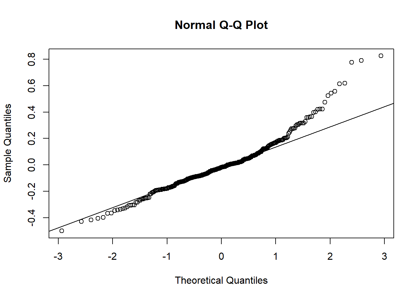
### QQ normal plot

qqnorm(resid)

qqline(resid)

#-----Remove variables w/ high p-values to see if it improves the model------

###Using backwards stepwise method

###If AIC goes UP by 2, it means the variable I took away was important. If it goes down by 2, the variable was not important

#___removed years2 because high p value___

test.fit<-lme(ch.cstock~ch.till+years+dep1+dep2+aquic+ipcc.soil+ipcc.pre+ipcc.temp,

              random = ~1|ran.exp/ran.yrexp, data = management.data, method = "ML", na.action = na.omit)

summary(test.fit)

Linear mixed-effects model fit by maximum likelihood
  Data: management.data 
       AIC       BIC   logLik
  -76.7991 -17.48534 54.39955

Random effects:
 Formula: ~1 | ran.exp
         (Intercept)
StdDev: 1.303409e-05

 Formula: ~1 | ran.yrexp %in% ran.exp
         (Intercept)  Residual
StdDev: 3.257696e-05 0.2019636

Fixed effects:  ch.cstock ~ ch.till + years + dep1 + dep2 + aquic + ipcc.soil +      ipcc.pre + ipcc.temp 
                      Value  Std.Error  DF   t-value p-value
(Intercept)       1.2125926 0.11932090 197 10.162449  0.0000
ch.tillrt        -0.0425056 0.02639774 197 -1.610199  0.1090
years             0.0024001 0.00176686  31  1.358386  0.1841
dep1             -0.0214085 0.00222589 197 -9.617962  0.0000
dep2              0.0002237 0.00002802 197  7.985297  0.0000
aquic            -0.0028738 0.04121330  60 -0.069731  0.9446
ipcc.soilham      0.0281122 0.10931122  60  0.257176  0.7979
ipcc.soillam     -0.0206449 0.11073860  60 -0.186429  0.8527
ipcc.soilsan     -0.0402531 0.23354192  60 -0.172359  0.8637
ipcc.soilspo     -0.0328137 0.23315511  60 -0.140738  0.8885
ipcc.soilwetland  0.0185992 0.11756895  60  0.158198  0.8748
ipcc.prewet       0.0890658 0.03070977  60  2.900245  0.0052
ipcc.tempwarm     0.0035184 0.03194056  60  0.110155  0.9127
 Correlation: 
                 (Intr) ch.tll years  dep1   dep2   aquic  ipcc.slh ipcc.sll
ch.tillrt         0.053                                                     
years            -0.174 -0.092                                              
dep1             -0.210 -0.099  0.040                                       
dep2              0.175  0.084 -0.083 -0.953                                
aquic             0.038 -0.051  0.103  0.039 -0.063                         
ipcc.soilham     -0.948 -0.106  0.024  0.051 -0.025 -0.069                  
ipcc.soillam     -0.877 -0.063  0.162  0.108 -0.066 -0.021  0.908           
ipcc.soilsan     -0.437 -0.014  0.070 -0.015  0.017  0.010  0.452    0.425  
ipcc.soilspo     -0.432 -0.011  0.040 -0.017  0.019  0.007  0.452    0.420  
ipcc.soilwetland -0.837 -0.075 -0.009  0.028 -0.003 -0.353  0.898    0.846  
ipcc.prewet      -0.259  0.043 -0.081 -0.208  0.192 -0.268  0.163   -0.021  
ipcc.tempwarm    -0.290 -0.044 -0.224  0.076 -0.087  0.023  0.226   -0.036  
                 ipcc.slsn ipcc.slsp ipcc.slw ipcc.p
ch.tillrt                                           
years                                               
dep1                                                
dep2                                                
aquic                                               
ipcc.soilham                                        
ipcc.soillam                                        
ipcc.soilsan                                        
ipcc.soilspo      0.217                             
ipcc.soilwetland  0.401     0.402                   
ipcc.prewet       0.035     0.038     0.146         
ipcc.tempwarm     0.109     0.116     0.092    0.279

Standardized Within-Group Residuals:
        Min          Q1         Med          Q3         Max 
-2.47927789 -0.59652632 -0.09190044  0.44295403  4.09368399 

Number of Observations: 301
Number of Groups: 
               ran.exp ran.yrexp %in% ran.exp 
                    69                    101 

### AIC went from -74 to -76, is that considered up or down in this case? I think down… so we keep years2?

###leaving out years2 because we want the model as simple as possible

#___removed ipcc.temp because high p value___

test.fit<-lme(ch.cstock~ch.till+years+dep1+dep2+aquic+ipcc.soil+ipcc.pre,

              random = ~1|ran.exp/ran.yrexp, data = management.data, method = "ML", na.action = na.omit)

summary(test.fit)

Linear mixed-effects model fit by maximum likelihood
  Data: management.data 
        AIC       BIC   logLik
  -78.78642 -23.17977 54.39321

Random effects:
 Formula: ~1 | ran.exp
        (Intercept)
StdDev: 8.53128e-06

 Formula: ~1 | ran.yrexp %in% ran.exp
         (Intercept)  Residual
StdDev: 3.132939e-05 0.2019678

Fixed effects:  ch.cstock ~ ch.till + years + dep1 + dep2 + aquic + ipcc.soil +      ipcc.pre 
                      Value  Std.Error  DF   t-value p-value
(Intercept)       1.2164087 0.11398593 197 10.671568  0.0000
ch.tillrt        -0.0423765 0.02632657 197 -1.609646  0.1091
years             0.0024438 0.00171885  31  1.421734  0.1651
dep1             -0.0214271 0.00221567 197 -9.670715  0.0000
dep2              0.0002240 0.00002786 197  8.039169  0.0000
aquic            -0.0029769 0.04113220  61 -0.072374  0.9425
ipcc.soilham      0.0253883 0.10629540  61  0.238846  0.8120
ipcc.soillam     -0.0202092 0.11047865  61 -0.182924  0.8555
ipcc.soilsan     -0.0430658 0.23174483  61 -0.185833  0.8532
ipcc.soilspo     -0.0358010 0.23117643  61 -0.154864  0.8774
ipcc.soilwetland  0.0174046 0.11686750  61  0.148926  0.8821
ipcc.prewet       0.0881233 0.02944326  61  2.992989  0.0040
 Correlation: 
                 (Intr) ch.tll years  dep1   dep2   aquic  ipcc.slh ipcc.sll
ch.tillrt         0.042                                                     
years            -0.257 -0.105                                              
dep1             -0.197 -0.096  0.059                                       
dep2              0.157  0.080 -0.106 -0.952                                
aquic             0.047 -0.050  0.111  0.038 -0.061                         
ipcc.soilham     -0.947 -0.098  0.078  0.034 -0.006 -0.076                  
ipcc.soillam     -0.928 -0.065  0.158  0.111 -0.070 -0.020  0.941           
ipcc.soilsan     -0.426 -0.009  0.097 -0.024  0.026  0.008  0.441    0.431  
ipcc.soilspo     -0.419 -0.006  0.068 -0.026  0.030  0.005  0.440    0.428  
ipcc.soilwetland -0.850 -0.072  0.012  0.021  0.005 -0.357  0.904    0.853  
ipcc.prewet      -0.194  0.058 -0.020 -0.240  0.226 -0.286  0.107   -0.011  
                 ipcc.slsn ipcc.slsp ipcc.slw
ch.tillrt                                    
years                                        
dep1                                         
dep2                                         
aquic                                        
ipcc.soilham                                 
ipcc.soillam                                 
ipcc.soilsan                                 
ipcc.soilspo      0.207                      
ipcc.soilwetland  0.395     0.396            
ipcc.prewet       0.005     0.006     0.125  

Standardized Within-Group Residuals:
        Min          Q1         Med          Q3         Max 
-2.47834042 -0.58885735 -0.09702779  0.43461959  4.09048124 

Number of Observations: 301
Number of Groups: 
               ran.exp ran.yrexp %in% ran.exp 
                    69                    101 

###changed AIC from -76 to -78, leaving out ipcc.temp

#____Removed aquic_____

test.fit<-lme(ch.cstock~ch.till+years+dep1+dep2+ipcc.soil+ipcc.pre,

              random = ~1|ran.exp/ran.yrexp, data = management.data, method = "ML", na.action = na.omit)

summary(test.fit)

Linear mixed-effects model fit by maximum likelihood
  Data: management.data 
       AIC      BIC  logLik
  -81.9712 -29.7498 54.9856

Random effects:
 Formula: ~1 | ran.exp
         (Intercept)
StdDev: 2.371439e-05

 Formula: ~1 | ran.yrexp %in% ran.exp
        (Intercept)  Residual
StdDev:  0.02037141 0.2014043

Fixed effects:  ch.cstock ~ ch.till + years + dep1 + dep2 + ipcc.soil + ipcc.pre 
                      Value  Std.Error  DF   t-value p-value
(Intercept)       1.3593818 0.08082279 203 16.819288  0.0000
ch.tillrt        -0.0433030 0.02635614 203 -1.642995  0.1019
years             0.0025717 0.00173446  31  1.482695  0.1483
dep1             -0.0211571 0.00217531 203 -9.726012  0.0000
dep2              0.0002207 0.00002743 203  8.044679  0.0000
ipcc.soilham     -0.1216511 0.06834101  63 -1.780060  0.0799
ipcc.soillam     -0.1647784 0.07512726  63 -2.193323  0.0320
ipcc.soilsan     -0.1894279 0.21724309  63 -0.871963  0.3865
ipcc.soilspo     -0.1826748 0.21655800  63 -0.843537  0.4021
ipcc.soilwetland -0.1319488 0.07341949  63 -1.797190  0.0771
ipcc.prewet       0.0868789 0.02875310  63  3.021548  0.0036
 Correlation: 
                 (Intr) ch.tll years  dep1   dep2   ipcc.slh ipcc.sll ipcc.slsn
ch.tillrt         0.060                                                        
years            -0.402 -0.100                                                 
dep1             -0.303 -0.089  0.053                                          
dep2              0.266  0.073 -0.097 -0.952                                   
ipcc.soilham     -0.891 -0.157  0.166  0.091 -0.070                            
ipcc.soillam     -0.849 -0.098  0.267  0.189 -0.149  0.869                     
ipcc.soilsan     -0.272 -0.010  0.115 -0.015  0.011  0.291    0.276            
ipcc.soilspo     -0.260 -0.007  0.083 -0.017  0.015  0.286    0.269    0.096   
ipcc.soilwetland -0.773 -0.143  0.112  0.083 -0.075  0.862    0.790    0.266   
ipcc.prewet      -0.276  0.047  0.013 -0.224  0.205  0.141   -0.026    0.006   
                 ipcc.slsp ipcc.slw
ch.tillrt                          
years                              
dep1                               
dep2                               
ipcc.soilham                       
ipcc.soillam                       
ipcc.soilsan                       
ipcc.soilspo                       
ipcc.soilwetland  0.263            
ipcc.prewet       0.006     0.036  

Standardized Within-Group Residuals:
        Min          Q1         Med          Q3         Max 
-2.71258136 -0.57976248 -0.08043712  0.43920736  4.07347191 

Number of Observations: 308
Number of Groups: 
               ran.exp ran.yrexp %in% ran.exp 
                    70                    102 

###Leaving out aquic because AIC changed from -78 to -81

#____removing ipcc.soil____

test.fit<-lme(ch.cstock~ch.till+years+dep1+dep2+ipcc.pre,

              random = ~1|ran.exp/ran.yrexp, data = management.data, method = "ML", na.action = na.omit)

summary(test.fit)

Linear mixed-effects model fit by maximum likelihood
  Data: management.data 
        AIC       BIC   logLik
  -87.44697 -53.87607 52.72348

Random effects:
 Formula: ~1 | ran.exp
        (Intercept)
StdDev:  0.01274511

 Formula: ~1 | ran.yrexp %in% ran.exp
        (Intercept)  Residual
StdDev:  0.04766797 0.1984883

Fixed effects:  ch.cstock ~ ch.till + years + dep1 + dep2 + ipcc.pre 
                 Value  Std.Error  DF  t-value p-value
(Intercept)  1.2155265 0.03673901 203 33.08544  0.0000
ch.tillrt   -0.0483838 0.02622587 203 -1.84489  0.0665
years        0.0037403 0.00174900  31  2.13852  0.0405
dep1        -0.0206351 0.00210659 203 -9.79550  0.0000
dep2         0.0002162 0.00002675 203  8.08192  0.0000
ipcc.prewet  0.0830077 0.02911534  68  2.85100  0.0058
 Correlation: 
            (Intr) ch.tll years  dep1   dep2  
ch.tillrt   -0.159                            
years       -0.545 -0.101                     
dep1        -0.432 -0.077 -0.017              
dep2         0.399  0.064 -0.045 -0.950       
ipcc.prewet -0.522  0.098  0.073 -0.165  0.154

Standardized Within-Group Residuals:
       Min         Q1        Med         Q3        Max 
-2.4822612 -0.5733692 -0.0913330  0.4402047  3.9800368 

Number of Observations: 308
Number of Groups: 
               ran.exp ran.yrexp %in% ran.exp 
                    70                    102 

###Leaving out ipcc.soil  because AIC changed from -81 to -87

#____removing ipcc.pre____*KEPT IPCC.PRE

test.fit<-lme(ch.cstock~ch.till+years+dep1+dep2,

              random = ~1|ran.exp/ran.yrexp, data = management.data, method = "ML", na.action = na.omit)

summary(test.fit)

Linear mixed-effects model fit by maximum likelihood
  Data: management.data 
        AIC       BIC   logLik
  -81.89104 -52.05024 48.94552

Random effects:
 Formula: ~1 | ran.exp
        (Intercept)
StdDev:  0.04089841

 Formula: ~1 | ran.yrexp %in% ran.exp
        (Intercept)  Residual
StdDev:   0.0410433 0.1994555

Fixed effects:  ch.cstock ~ ch.till + years + dep1 + dep2 
                 Value  Std.Error  DF  t-value p-value
(Intercept)  1.2772696 0.03284326 203 38.88985  0.0000
ch.tillrt   -0.0567931 0.02661311 203 -2.13403  0.0340
years        0.0031722 0.00182699  31  1.73630  0.0924
dep1        -0.0200671 0.00210794 203 -9.51980  0.0000
dep2         0.0002095 0.00002674 203  7.83402  0.0000
 Correlation: 
          (Intr) ch.tll years  dep1  
ch.tillrt -0.138                     
years     -0.602 -0.088              
dep1      -0.611 -0.059  0.011       
dep2       0.564  0.049 -0.071 -0.949

Standardized Within-Group Residuals:
       Min         Q1        Med         Q3        Max 
-2.3393973 -0.5998968 -0.1325983  0.4353780  3.9937867 

Number of Observations: 308
Number of Groups: 
               ran.exp ran.yrexp %in% ran.exp 
                    70                    102 

### Keeping ipcc.pre because AIC changed from -87 back to -81

#----Best Fit Management Model-----

test.fit.management<-lme(ch.cstock~ch.till+years+dep1+dep2+ipcc.pre,

              random = ~1|ran.exp/ran.yrexp, data = management.data, method = "ML", na.action = na.omit)

summary(test.fit.management)

Linear mixed-effects model fit by maximum likelihood
  Data: management.data 
        AIC       BIC   logLik
  -87.44697 -53.87607 52.72348

Random effects:
 Formula: ~1 | ran.exp
        (Intercept)
StdDev:  0.01274511

 Formula: ~1 | ran.yrexp %in% ran.exp
        (Intercept)  Residual
StdDev:  0.04766797 0.1984883

Fixed effects:  ch.cstock ~ ch.till + years + dep1 + dep2 + ipcc.pre 
                 Value  Std.Error  DF  t-value p-value
(Intercept)  1.2155265 0.03673901 203 33.08544  0.0000
ch.tillrt   -0.0483838 0.02622587 203 -1.84489  0.0665
years        0.0037403 0.00174900  31  2.13852  0.0405
dep1        -0.0206351 0.00210659 203 -9.79550  0.0000
dep2         0.0002162 0.00002675 203  8.08192  0.0000
ipcc.prewet  0.0830077 0.02911534  68  2.85100  0.0058
 Correlation: 
            (Intr) ch.tll years  dep1   dep2  
ch.tillrt   -0.159                            
years       -0.545 -0.101                     
dep1        -0.432 -0.077 -0.017              
dep2         0.399  0.064 -0.045 -0.950       
ipcc.prewet -0.522  0.098  0.073 -0.165  0.154

Standardized Within-Group Residuals:
       Min         Q1        Med         Q3        Max 
-2.4822612 -0.5733692 -0.0913330  0.4402047  3.9800368 

Number of Observations: 308
Number of Groups: 
               ran.exp ran.yrexp %in% ran.exp 
                    70                    102 

#____________________________________________________________________________________________________________

  #cINPUT MODEL DEVELOPMENT

#-------Test full model with all variables as main effects-------

###Did not include soil type because it does not matter for Cinput data

test.fit<-lme(ch.cstock~ch.inp+years+years2+dep1+dep2+aquic+ipcc.pre+ipcc.temp,

              random = ~1|ran.exp/ran.yrexp, data = Cinput.data, method = "ML", na.action = na.omit)

summary(test.fit)

Linear mixed-effects model fit by maximum likelihood
  Data: Cinput.data 
        AIC       BIC   logLik
  -218.2465 -186.1726 121.1233

Random effects:
 Formula: ~1 | ran.exp
        (Intercept)
StdDev:  0.02133355

 Formula: ~1 | ran.yrexp %in% ran.exp
         (Intercept)   Residual
StdDev: 1.165634e-06 0.07551378

Fixed effects:  ch.cstock ~ ch.inp + years + years2 + dep1 + dep2 + aquic + ipcc.pre +      ipcc.temp 
                   Value  Std.Error DF   t-value p-value
(Intercept)    1.0613041 0.04821888 58 22.010133  0.0000
ch.inpl       -0.1273723 0.02700289 58 -4.716987  0.0000
years         -0.0031645 0.00403780 22 -0.783723  0.4416
years2         0.0000647 0.00009054 22  0.714163  0.4826
dep1           0.0031662 0.00151394 58  2.091352  0.0409
dep2          -0.0000222 0.00001901 58 -1.170089  0.2468
aquic         -0.0509499 0.08979628 18 -0.567394  0.5775
ipcc.prewet    0.0206511 0.02953017 18  0.699321  0.4933
ipcc.tempwarm -0.0239228 0.02288024 18 -1.045567  0.3096
 Correlation: 
              (Intr) ch.npl years  years2 dep1   dep2   aquic  ipcc.p
ch.inpl       -0.652                                                 
years         -0.780  0.272                                          
years2         0.731 -0.289 -0.974                                   
dep1          -0.270  0.044 -0.016 -0.019                            
dep2           0.244 -0.033  0.012  0.013 -0.957                     
aquic          0.128  0.103 -0.233  0.186  0.070 -0.049              
ipcc.prewet   -0.509  0.503  0.360 -0.324 -0.156  0.150 -0.166       
ipcc.tempwarm -0.170 -0.189  0.097 -0.015  0.058 -0.080 -0.182 -0.268

Standardized Within-Group Residuals:
        Min          Q1         Med          Q3         Max 
-2.24478048 -0.54906957 -0.01933017  0.50813897  3.33744254 

Number of Observations: 107
Number of Groups: 
               ran.exp ran.yrexp %in% ran.exp 
                    22                     46 

#____Removing aquic because high p value____

test.fit<-lme(ch.cstock~ch.inp+years+years2+dep1+dep2+ipcc.pre+ipcc.temp,

              random = ~1|ran.exp/ran.yrexp, data = Cinput.data, method = "ML", na.action = na.omit)

summary(test.fit)

Linear mixed-effects model fit by maximum likelihood
  Data: Cinput.data 
        AIC       BIC   logLik
  -219.8959 -190.4948 120.9479

Random effects:
 Formula: ~1 | ran.exp
        (Intercept)
StdDev:  0.02155949

 Formula: ~1 | ran.yrexp %in% ran.exp
         (Intercept)   Residual
StdDev: 1.404757e-06 0.07559902

Fixed effects:  ch.cstock ~ ch.inp + years + years2 + dep1 + dep2 + ipcc.pre +      ipcc.temp 
                   Value  Std.Error DF   t-value p-value
(Intercept)    1.0647743 0.04770339 58 22.320728  0.0000
ch.inpl       -0.1257814 0.02679209 58 -4.694723  0.0000
years         -0.0036977 0.00391837 22 -0.943685  0.3556
years2         0.0000742 0.00008879 22  0.835624  0.4124
dep1           0.0032287 0.00150467 58  2.145753  0.0361
dep2          -0.0000228 0.00001891 58 -1.205032  0.2331
ipcc.prewet    0.0178249 0.02907533 19  0.613060  0.5471
ipcc.tempwarm -0.0262489 0.02247104 19 -1.168122  0.2572
 Correlation: 
              (Intr) ch.npl years  years2 dep1   dep2   ipcc.p
ch.inpl       -0.674                                          
years         -0.777  0.306                                   
years2         0.725 -0.315 -0.974                            
dep1          -0.281  0.037  0.000 -0.033                     
dep2           0.252 -0.027  0.001  0.022 -0.957              
ipcc.prewet   -0.498  0.529  0.335 -0.302 -0.146  0.144       
ipcc.tempwarm -0.150 -0.173  0.057  0.020  0.072 -0.090 -0.308

Standardized Within-Group Residuals:
        Min          Q1         Med          Q3         Max 
-2.24054950 -0.55163767 -0.06600909  0.52227609  3.36081396 

Number of Observations: 107
Number of Groups: 
               ran.exp ran.yrexp %in% ran.exp 
                    22                     46 

###Leave out aquic

#____Removing ipcc.pre_____

test.fit<-lme(ch.cstock~ch.inp+years+years2+dep1+dep2+ipcc.temp,

              random = ~1|ran.exp/ran.yrexp, data = Cinput.data, method = "ML", na.action = na.omit)

summary(test.fit)

Linear mixed-effects model fit by maximum likelihood
  Data: Cinput.data 
        AIC       BIC   logLik
  -221.5017 -194.7734 120.7508

Random effects:
 Formula: ~1 | ran.exp
        (Intercept)
StdDev:  0.02279106

 Formula: ~1 | ran.yrexp %in% ran.exp
         (Intercept)   Residual
StdDev: 6.608399e-07 0.07549399

Fixed effects:  ch.cstock ~ ch.inp + years + years2 + dep1 + dep2 + ipcc.temp 
                   Value  Std.Error DF   t-value p-value
(Intercept)    1.0787360 0.04157504 58 25.946720  0.0000
ch.inpl       -0.1341617 0.02286890 58 -5.866557  0.0000
years         -0.0044796 0.00371354 22 -1.206295  0.2405
years2         0.0000901 0.00008522 22  1.056801  0.3021
dep1           0.0033722 0.00148184 58  2.275709  0.0266
dep2          -0.0000246 0.00001862 58 -1.318874  0.1924
ipcc.tempwarm -0.0217812 0.02160346 20 -1.008228  0.3254
 Correlation: 
              (Intr) ch.npl years  years2 dep1   dep2  
ch.inpl       -0.558                                   
years         -0.748  0.162                            
years2         0.695 -0.193 -0.972                     
dep1          -0.408  0.131  0.054 -0.083              
dep2           0.372 -0.119 -0.051  0.069 -0.956       
ipcc.tempwarm -0.370 -0.010  0.175 -0.077  0.028 -0.047

Standardized Within-Group Residuals:
        Min          Q1         Med          Q3         Max 
-2.21678502 -0.58798692 -0.06059058  0.50893876  3.21488084 

Number of Observations: 107
Number of Groups: 
               ran.exp ran.yrexp %in% ran.exp 
                    22                     46 

###Leave out ipcc.pre

#_____Removing ipcc.temp____

test.fit<-lme(ch.cstock~ch.inp+years+years2+dep1+dep2,

              random = ~1|ran.exp/ran.yrexp, data = Cinput.data, method = "ML", na.action = na.omit)

summary(test.fit)

Linear mixed-effects model fit by maximum likelihood
  Data: Cinput.data 
        AIC       BIC   logLik
  -222.4738 -198.4183 120.2369

Random effects:
 Formula: ~1 | ran.exp
        (Intercept)
StdDev:  0.02537353

 Formula: ~1 | ran.yrexp %in% ran.exp
         (Intercept)   Residual
StdDev: 3.806715e-07 0.07533366

Fixed effects:  ch.cstock ~ ch.inp + years + years2 + dep1 + dep2 
                 Value  Std.Error DF   t-value p-value
(Intercept)  1.0624051 0.03926304 58 27.058654  0.0000
ch.inpl     -0.1336006 0.02330449 58 -5.732826  0.0000
years       -0.0038257 0.00372994 22 -1.025661  0.3162
years2       0.0000831 0.00008682 22  0.956987  0.3490
dep1         0.0034261 0.00147686 58  2.319843  0.0239
dep2        -0.0000255 0.00001852 58 -1.379507  0.1730
 Correlation: 
        (Intr) ch.npl years  years2 dep1  
ch.inpl -0.603                            
years   -0.750  0.167                     
years2   0.721 -0.195 -0.976              
dep1    -0.418  0.120  0.052 -0.082       
dep2     0.372 -0.109 -0.044  0.066 -0.956

Standardized Within-Group Residuals:
        Min          Q1         Med          Q3         Max 
-2.11617924 -0.62191195 -0.03337844  0.53035651  3.11400864 

Number of Observations: 107
Number of Groups: 
               ran.exp ran.yrexp %in% ran.exp 
                    22                     46 

#only brought down AIC by 1, might keep out? Means it really has no affect on the model, but we want the model as simple as possible anyway.

###NOTE: Taking out years2 because it worsened the model

#----Best Fit C Input Model-----

test.fit.CInput<-lme(ch.cstock~ch.inp+years+dep1+dep2,

              random = ~1|ran.exp/ran.yrexp, data = Cinput.data, method = "REML", na.action = na.omit)

summary(test.fit.CInput)

Linear mixed-effects model fit by REML
  Data: Cinput.data 
        AIC       BIC   logLik
  -164.3576 -143.3578 90.17879

Random effects:
 Formula: ~1 | ran.exp
        (Intercept)
StdDev:    0.030629

 Formula: ~1 | ran.yrexp %in% ran.exp
         (Intercept)   Residual
StdDev: 3.188172e-07 0.07654272

Fixed effects:  ch.cstock ~ ch.inp + years + dep1 + dep2 
                 Value   Std.Error DF  t-value p-value
(Intercept)  1.0342824 0.027920709 58 37.04356  0.0000
ch.inpl     -0.1280234 0.023610778 58 -5.42224  0.0000
years       -0.0003797 0.000856623 23 -0.44328  0.6617
dep1         0.0035614 0.001463052 58  2.43426  0.0180
dep2        -0.0000268 0.000018323 58 -1.46459  0.1484
 Correlation: 
        (Intr) ch.npl years  dep1  
ch.inpl -0.675                     
years   -0.330 -0.099              
dep1    -0.492  0.086 -0.122       
dep2     0.444 -0.080  0.090 -0.956

Standardized Within-Group Residuals:
        Min          Q1         Med          Q3         Max 
-2.10382963 -0.55572607  0.02143947  0.53793687  3.08551597 

Number of Observations: 107
Number of Groups: 
               ran.exp ran.yrexp %in% ran.exp 
                    22                     46 

#________________________________________________________________________________________________

  #LAND USE MODEL DEVELOPMENT

#-------Test full model with all variables as main effects-------

###Did not include soil type pr aquic because it does not matter for Cinput data because we did not have enough soil type representation or aquic sites to fully represent the model

test.fit<-lme(ch.cstock~years+years2+dep1+dep2+ipcc.prec+ipcc.temp,

              random = ~1|ran.exp/ran.yrexp, data = LU.data, method = "ML", na.action = na.omit)

summary(test.fit)

Linear mixed-effects model fit by maximum likelihood
  Data: LU.data 
      AIC      BIC   logLik
  10.1963 39.75457 4.901848

Random effects:
 Formula: ~1 | ran.exp
        (Intercept)
StdDev:  0.07900865

 Formula: ~1 | ran.yrexp %in% ran.exp
        (Intercept) Residual
StdDev: 2.80147e-05  0.22315

Fixed effects:  ch.cstock ~ years + years2 + dep1 + dep2 + ipcc.prec + ipcc.temp 
                   Value  Std.Error DF   t-value p-value
(Intercept)    0.8533453 0.08722319 93  9.783468  0.0000
years         -0.0081524 0.00280862  9 -2.902638  0.0175
years2         0.0000594 0.00002376  9  2.500383  0.0338
dep1           0.0168374 0.00290466 93  5.796695  0.0000
dep2          -0.0001320 0.00003254 93 -4.056438  0.0001
ipcc.precwet  -0.0481100 0.06114358  9 -0.786836  0.4516
ipcc.tempwarm -0.0873289 0.05283942  9 -1.652722  0.1328
 Correlation: 
              (Intr) years  years2 dep1   dep2   ipcc.p
years         -0.752                                   
years2         0.677 -0.953                            
dep1          -0.294 -0.074  0.055                     
dep2           0.234  0.042 -0.028 -0.916              
ipcc.precwet  -0.484  0.414 -0.448 -0.130  0.109       
ipcc.tempwarm -0.386 -0.030 -0.016  0.098 -0.026  0.172

Standardized Within-Group Residuals:
        Min          Q1         Med          Q3         Max 
-2.69345778 -0.68525693 -0.07894826  0.48777740  3.48592852 

Number of Observations: 142
Number of Groups: 
               ran.exp ran.yrexp %in% ran.exp 
                    34                     47 

#____Remove ipcc.prec____

test.fit<-lme(ch.cstock~years+years2+dep1+dep2+ipcc.temp,

              random = ~1|ran.exp/ran.yrexp, data = LU.data, method = "ML", na.action = na.omit)

summary(test.fit)

Linear mixed-effects model fit by maximum likelihood
  Data: LU.data 
       AIC      BIC   logLik
  8.845024 35.44747 4.577488

Random effects:
 Formula: ~1 | ran.exp
        (Intercept)
StdDev:  0.08019223

 Formula: ~1 | ran.yrexp %in% ran.exp
         (Intercept) Residual
StdDev: 1.994477e-05 0.223438

Fixed effects:  ch.cstock ~ years + years2 + dep1 + dep2 + ipcc.temp 
                   Value  Std.Error DF   t-value p-value
(Intercept)    0.8200451 0.07637270 93 10.737411  0.0000
years         -0.0072352 0.00255963 10 -2.826678  0.0180
years2         0.0000510 0.00002127 10  2.397972  0.0374
dep1           0.0165354 0.00287370 93  5.754030  0.0000
dep2          -0.0001292 0.00003228 93 -4.003265  0.0001
ipcc.tempwarm -0.0800712 0.05215433 10 -1.535275  0.1557
 Correlation: 
              (Intr) years  years2 dep1   dep2  
years         -0.693                            
years2         0.588 -0.944                     
dep1          -0.410 -0.023 -0.003              
dep2           0.329 -0.003  0.023 -0.915       
ipcc.tempwarm -0.350 -0.113  0.069  0.123 -0.046

Standardized Within-Group Residuals:
        Min          Q1         Med          Q3         Max 
-2.65812143 -0.68568772 -0.05351942  0.53865794  3.50204247 

Number of Observations: 142
Number of Groups: 
               ran.exp ran.yrexp %in% ran.exp 
                    34                     47 

###Keep ipcc.pre out

#____Remove ipcc.temp____

test.fit<-lme(ch.cstock~years+years2+dep1+dep2,

              random = ~1|ran.exp/ran.yrexp, data = LU.data, method = "ML", na.action = na.omit)

summary(test.fit)

Linear mixed-effects model fit by maximum likelihood
  Data: LU.data 
       AIC      BIC   logLik
  9.159036 32.80565 3.420482

Random effects:
 Formula: ~1 | ran.exp
        (Intercept)
StdDev:  0.09172667

 Formula: ~1 | ran.yrexp %in% ran.exp
         (Intercept)  Residual
StdDev: 1.628889e-05 0.2227962

Fixed effects:  ch.cstock ~ years + years2 + dep1 + dep2 
                 Value  Std.Error DF   t-value p-value
(Intercept)  0.7804414 0.07372605 93 10.585695  0.0000
years       -0.0076584 0.00262714 11 -2.915094  0.0141
years2       0.0000529 0.00002195 11  2.412040  0.0345
dep1         0.0169964 0.00284137 93  5.981773  0.0000
dep2        -0.0001316 0.00003215 93 -4.092387  0.0001
 Correlation: 
       (Intr) years  years2 dep1  
years  -0.788                     
years2  0.653 -0.943              
dep1   -0.379 -0.012 -0.009       
dep2    0.321 -0.006  0.023 -0.915

Standardized Within-Group Residuals:
        Min          Q1         Med          Q3         Max 
-2.75464698 -0.69354075 -0.06667757  0.56532555  3.53624701 

Number of Observations: 142
Number of Groups: 
               ran.exp ran.yrexp %in% ran.exp 
                    34                     47 

###Leave out ipcc.temp, AIC only changed by 1 so it has no significant effects on the model

#----Best Fit Land Use Model----

test.fit.LU<-lme(ch.cstock~years+years2+dep1+dep2,

              random = ~1|ran.exp/ran.yrexp, data = LU.data, method = "ML", na.action = na.omit)

summary(test.fit.LU)

Linear mixed-effects model fit by maximum likelihood
  Data: LU.data 
       AIC      BIC   logLik
  9.159036 32.80565 3.420482

Random effects:
 Formula: ~1 | ran.exp
        (Intercept)
StdDev:  0.09172667

 Formula: ~1 | ran.yrexp %in% ran.exp
         (Intercept)  Residual
StdDev: 1.628889e-05 0.2227962

Fixed effects:  ch.cstock ~ years + years2 + dep1 + dep2 
                 Value  Std.Error DF   t-value p-value
(Intercept)  0.7804414 0.07372605 93 10.585695  0.0000
years       -0.0076584 0.00262714 11 -2.915094  0.0141
years2       0.0000529 0.00002195 11  2.412040  0.0345
dep1         0.0169964 0.00284137 93  5.981773  0.0000
dep2        -0.0001316 0.00003215 93 -4.092387  0.0001
 Correlation: 
       (Intr) years  years2 dep1  
years  -0.788                     
years2  0.653 -0.943              
dep1   -0.379 -0.012 -0.009       
dep2    0.321 -0.006  0.023 -0.915

Standardized Within-Group Residuals:
        Min          Q1         Med          Q3         Max 
-2.75464698 -0.69354075 -0.06667757  0.56532555  3.53624701 

Number of Observations: 142
Number of Groups: 
               ran.exp ran.yrexp %in% ran.exp 
                    34                     47 

#______________________________________________________________________________________________

### EF'S THEN CALCULATED IN EXCEL

# Derive PDF for each model/EF

###Land Use EF

fixed.LU<-fixed.effects(test.fit.LU)

LU.cov<-test.fit.LU$varFix

x.LU<-c(1,75,5625,15,300)

# Variance

V.LU.EF<-(t(x.LU))%*%LU.cov%*%x.LU

# Standard Deviation

sqrt(V.LU.EF)

           [,1]
[1,] 0.03887679

#_________________________________________

###CInput EF

fixed.Cinput<-fixed.effects(test.fit.CInput)

Cinput.cov<-test.fit.CInput$varFix

X.Cinput.low<-c(1,1,75,15,300)

X.Cinput.high<-c(1,0,75,15,300)

# Variance

V.Cinput.low<-(t(X.Cinput.low))%*%Cinput.cov%*%X.Cinput.low

V.Cinput.high<-(t(X.Cinput.high))%*%Cinput.cov%*%X.Cinput.high

# Standard Deviation

sqrt(V.Cinput.low)

           [,1]
[1,] 0.05190687

sqrt(V.Cinput.high)

           [,1]
[1,] 0.05707304

#_________________________________________

###Management EF

fixed.management<-fixed.effects(test.fit.management)

management.cov<-test.fit.management$varFix

x.rt.wet<-c(1,1,20,15,300,1)

x.nt.wet<-c(1,0,20,15,300,1)

x.nt.dry<-c(1,0,20,15,300,0)

x.rt.dry<-c(1,1,20,15,300,0)

# Variance

v.rt.wet<-(t(x.rt.wet))%*%management.cov%*%x.rt.wet

v.nt.wet<-(t(x.nt.wet))%*%management.cov%*%x.nt.wet

v.nt.dry<-(t(x.nt.dry))%*%management.cov%*%x.nt.dry

v.rt.dry<-(t(x.rt.dry))%*%management.cov%*%x.rt.dry

# Standard Deviation

sqrt(v.rt.wet)

           [,1]
[1,] 0.02827946

sqrt(v.nt.wet)

           [,1]
[1,] 0.02364594

sqrt(v.nt.dry)

           [,1]
[1,] 0.03007006

sqrt(v.rt.dry)

           [,1]
[1,] 0.03158836

#_____________Export CSV files with my covariance matrix to run in cholesky decomp model for monte carlo__________________

###CSV files

#write.csv(data.frame(LU.cov), "LandUseCov.csv")

#write.csv(data.frame(Cinput.cov), "CinputCov.csv")

#write.csv(data.frame(management.cov), "MgmtCov.csv")

#NOTE: always keep dep1 and dep2 when testing the model w/ AIC value and years